Explore and analyze graphs in Garphield

Navigate and find nodes

Drag the canvas to pan. Use a wheel, touchpad, or pinch gesture to zoom. Press / to search by node label or id.

Use pointer, marquee, or lasso selection. To inspect a route, select exactly one source node, choose Pick path target in the bottom control bar, then click an actual target node. Garphield emphasizes the exact shortest path, following link direction on directed networks. Clicking empty canvas or a node with no directed route leaves target mode active so you can try again.

Choose the Microscope button immediately to its right to turn on the fisheye lens. Move the pointer to magnify local structure without losing the surrounding network, then click to pin it. Clicking empty canvas moves the lens to that location with a short glide; clicking a node glides to and centers exactly on the node. A pinned lens shows a subtle inner grab ring: drag that ring past its short resistance to release the lens back to pointer-following. The center stays available for moving the network or selected nodes. Press Esc to release it without dragging; touch layouts also show an unpin button at the lens’s upper right. Hover the outer boundary to reveal resize handles, then drag that boundary with the primary button to resize it. Right-drag up or down inside the circle to change magnification. Wheel, touchpad, and pinch gestures continue to zoom the canvas everywhere, including inside the lens. For keyboard access, focus the Microscope button and use the arrow keys to adjust magnification. The glide is disabled when reduced motion is requested.

Temporarily hide nodes

Select one or more nodes, then choose Hide in the selection toolbar. On a phone, tap a node and choose Hide node in its Info details. On desktop, you can also right-click a node and choose Hide node. Right-click a selected node to hide the whole selection. Choose Keep only selected to hide all other visible nodes; this creates a separate group and preserves existing hides and filters. The action is also available in the phone’s Info details.

The hidden count on the canvas opens the hidden groups in Sets (or the phone’s Info sheet). Hides within three seconds join one group and one undo step. A pause, another edit, a restore, or a pinned history point starts a new group. Rename a group and add a note to remember why you hid it. A notification reports how many nodes changed and offers Undo.

Search within a group to restore individual nodes, check several and choose Restore selected, restore a whole group with its eye button, or choose Restore all. Incident edges return too, subject to active filters. Restored groups keep their membership so you can hide them again, or drag them onto a visual channel. Deleting a group also restores its nodes.

Hide and restore support Undo/Redo and history navigation. Groups and their visibility are preserved in saved/shared views and .gph sessions. Loading a new graph clears the previous graph’s sets. Hiding keeps source data and node positions intact. Use Zoom to fit after moving or hiding nodes to frame the remaining visible nodes at their current positions. Fit preserves rotation and can be undone without moving the nodes.

Community detection, centrality, and graph statistics run on the visible graph: hidden nodes and hidden edges are excluded, while faded elements remain included. The app evaluates filter predicates before analyzing their output, so a degree filter remains stable when the visible graph’s degrees change. Automatic drawing simplifications such as backbone views do not change this analysis topology.

Save sets

Open Sets to name the current selection. A saved set can be selected again, used in a filter, assigned to a visual channel, or included in a Story step.

Encode and filter

Open Explore in the Viz panel. Drag a source into a compatible visual channel.

Source result	Examples	Visual channels
Number	Degree, Betweenness, weight	Size, colour, link width, heatmap
Category	Louvain, Leiden, text fields	Colour, shape, contour
Set	Selection, saved set, path, bridges	Border and set emphasis

Use Style for base node, link, label, and canvas appearance. Node surfaces can be Flat, softly lit with Lumen, fully round with Sphere, faceted with Prism, or hand-drawn with Sketchy. Sphere keeps node images and shades them as spherical textures; the other modes continue to respect the node’s data-driven fill. Filters accept numeric ranges, categories, dates, and sets. Fade retains context; Hide removes non-matching elements from the view. Filtering preserves the graph’s data, topology, and node positions.

Share URLs preserve the complete visible style: node surface and size, node gap, link width and opacity, curvature, labels, link direction and gradient, theme, and the fisheye’s enabled state, magnification, and radius. The lens focus itself is transient and is not saved.

Explore a network over time

Try File → Data library → Collaboration over time, a synthetic network with six weeks of dates. In Viz, use the Filter card above Node marks to choose joined and reveal nodes as they join, or collaborated to reveal edges as collaborations happen. The funnel adds another filter. Browse lists node and edge fields first. Date fields have a clock badge and can also be used as categories in visual channels.

• The histogram shows how dates are distributed over time. Drag its upper handle to reveal values as of that instant. Drag the lower handle inward to select a date window; return it to the beginning to remove the start bound.
• Click the date readout below the histogram to edit exact UTC dates, then press Enter to apply each date. Both boundaries are inclusive.
• Use previous/next to step through distinct timestamps, or Play to advance the end date. For large timelines, 1× covers the selected date range in about 20 seconds, 5× in about 4 seconds, and 20× in about one second. Playback batches dates when needed; previous/next still visits every date. A selected start date stays fixed. Gaps without events do not slow playback.
• The same button becomes Pause during playback. Reset returns to the earliest date, and Loop restarts from the start date at the end. Play at the end also replays from the start. Playback pauses when the tab is hidden, the filter is disabled or removed, the data changes, or a saved view is restored.

Dates must be YYYY-MM-DD (UTC midnight) or an RFC3339 timestamp with an explicit timezone, such as 2026-01-05T12:30:00Z or 2026-01-05T13:30:00+01:00. Seconds and milliseconds are preserved in the displayed cursor when needed. Numeric epochs, locale dates, and timestamps without a timezone are not inferred. Date-only end values mean midnight; use the next date or an explicit time when you want to include events later in a day.

Time filters hide excluded nodes and edges by default; the filter mode control can switch to fading them as context.

Every nonempty value in a field must be a valid date for automatic detection. Empty values are reported and excluded by default. Show undated nodes/edges includes them as context. Undated nodes need a connection to dated nodes in the window; disconnected timeless components stay excluded. If an existing temporal field gains an invalid value, its filter becomes unavailable until the value is corrected; the graph is left unfiltered by that row. The match count describes this field’s date range, before other filters are combined.

Node date filters also affect incident edges. Edge date filters exclude nodes without a connection in the window, so future nodes do not appear as orphans. Shared URLs, .gph files, and captured Story steps preserve both date bounds and the undated-value choice. Playback speed and looping are local controls and do not autoplay when opening a saved view. Hide date filters also narrow the topology used for community detection and statistics; Fade date filters leave it intact.

Analyze

Garphield runs network algorithms in the browser. Common sources include:

• Degree, Betweenness, Closeness, PageRank, Eigenvector, Harmonic, and Katz centrality;
• Louvain, Leiden, label propagation, greedy modularity, and K-clique communities;
• shortest paths, ego networks, reachability, K-core, bridges, and articulation points; and
• link measures including Betweenness, Jaccard, and Adamic–Adar.

Bind an algorithm result, filter with it, inspect its values in the table, or reuse it later in the pipeline. See Sources and algorithms for the full catalogue.

Transform or generate a network

Transformations extract structures such as the largest component, a spanning tree, a K-core, or a disparity-filter backbone. Each transformation becomes a reversible pipeline step and can feed later algorithms.

Choose File → Generate for reproducible random, small-world, scale-free, tree, grid, cycle, star, wheel, barbell, or bipartite networks.

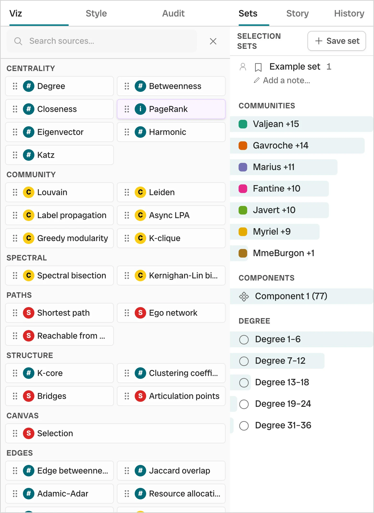
1. 1Explore catalogue
2. 2Sets panel

Sources and saved sets can be reused across the pipeline.

Use History to reverse or compare any selection, binding, filter, transformation, or generated network.

Layout animation

Asynchronous Force layouts reveal moving nodes by default. Connected nodes flock together, then decelerate into the completed layout over about 1.7 seconds. Links then grow into view over 0.6 seconds. Levels moves directly to its completed layout without this animation. Reduced-motion preferences also disable the animation. Cancelling a layout or loading another graph cancels its preview.

For layouts above 5,000 nodes or 20,000 edges, a preparation indicator can appear before the animation begins. It clears while the animation is running.

Graphs open in Full view. Backbone and Onion remain available as explicit choices, and saved views retain the chosen presentation.