Interactive NetworkX graph visualization in Jupyter

Part 1 of Python to workbench and back.

NetworkX supplies the graph and initial calculations. Garphield supplies the interactive view.

Build the graph

uv pip install 'garphield[networkx]'

import garphield as gph
import networkx as nx

graph = nx.les_miserables_graph()
communities = nx.community.greedy_modularity_communities(graph, weight="weight")

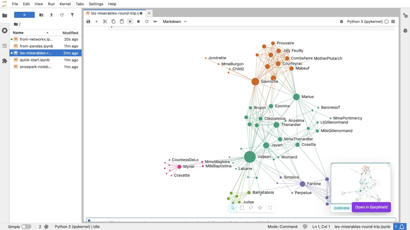
view = gph.show(
    graph,
    node_size=graph.degree,
    node_color=communities,
    node_label=str,
    layout="force",
    height=640,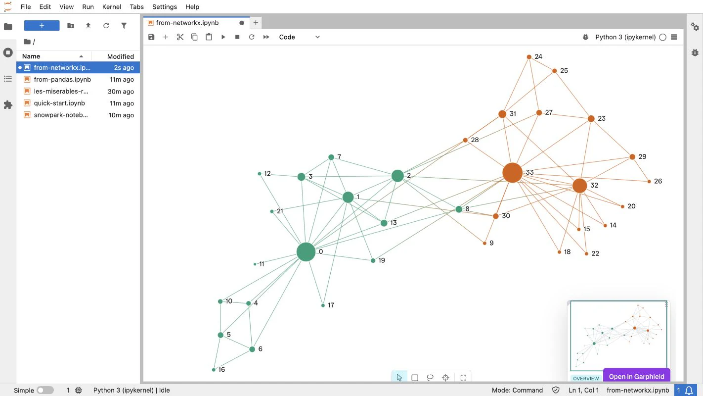
)

NetworkX degree controls size; the community partition controls colour.

Change the view from Python

The same GraphView accepts later changes:

view.bind("node_color", gph.algorithm("louvain", resolution=1.1))
view.fit()

Attribute names, mappings, degree views, sets, partitions, and callables can all become visual bindings.

The view stays beside the code that constructed the graph.

React to selection

def report_selection(nodes):
    print(f"Selected: {nodes}")

unsubscribe = view.on_selection(report_selection)

Use the callback to join selected identities to another table, inspect a model, or record a decision in the notebook.

Read the project back

edited = view.to_project()
edited_graph = view.to_networkx()

edited.save("les-miserables-notebook.gph")

The project carries graph data and the visual work. Continue with Refine the view to open it in the full workbench.